4  The Madison Square Garden Effect in the NBA

Author

Robert Hutto

4.1 The Madison Square Garden Effect in the NBA

4.1.1 What is Madison Square Garden?

MSG, or “The Garden”, is a historic arena located in the heart of Manhattan. The Garden opened on February 11, 1968, making it the oldest major sporting facility in the New York metropolitan area and the oldest active arena in the NBA. Beyond basketball, the arena hosts concerts, boxing matches, political events, and other major cultural performances, making it one of the most recognizable venues in the world. The Garden is especially iconic in the world of basketball, with many revering it as the “Mecca of Basketball”.

4.1.2 What makes MSG so special?

MSG is the premier indoor venue of New York City–the most visited and densely populated city in the United States, as well as the nation’s largest media market. Events held at MSG often receive disproportionate national and international attention, and NBA games played at The Garden are more likely to be nationally televised, widely discussed in sports media, and preserved in highlight compilations than games played elsewhere.

MSG is also the home court of the New York Knicks, one of the NBA’s most valuable and widely followed franchises, regardless of on-court success. Knicks fans are notoriously vocal, expressive, and unafraid to engage with players. Courtside seats are typically filled with famous actors, musicians, athletes, and public figures, many of whom are highlighted on broadcasts and arena displays. On any given night, there are dozens of high-profile celebrities present throughout the arena, creating a feeling that the game is a public showcase, rather than just another regular-season game. Given the arena’s historic status, visibility, and the fans it brings in, performances at MSG are perceived as particularly meaningful and memorable.

In line with this, MSG boasts a long list of iconic player performances. Michael Jordan scored 55 points in his “double-nickel” return game to MSG on March 28, 1995 after his first retirement, definitively reinstating himself as the face of the league. On February 2, 2009, Kobe Bryant set the record for most points scored in a game at The Garden with a 61-point performance, solidifying his legacy as one of the best scorers the NBA has ever seen. Stephen Curry’s breakout game on February 27, 2013, where he made 11 out of his 13 three-point attempts to score 54 points at The Garden, is often referenced as the moment he elevated to star status. Nearly nine years later at The Garden, Curry hit his 2974th career three-pointer, surpassing Ray Allen and breaking the NBA’s all-time three point scoring record. The list goes on.

This combination of historical performances, celebrity presence, media visibility, and competitive intensity has brought on a widely-accepted narrative that the pressures associated with MSG uniquely influence individual games and player performances. Clutch star players rise to the occasion with standout performances, while others “shrink under the lights” and struggle to perform, further entrenching the belief that the arena itself exerts an influence on performance.

4.1.3 Is the MSG effect real?

While perceptions of the “MSG Effect” are deeply ingrained in basketball culture, they are rooted in isolated moments, media framing, and retrospective storytelling rather than statistics. The present analysis seeks to address this gap by examining whether this “MSG Effect” is actually detectable in statistics, or if it is simply a product of our narrative-obsessed imagination.

4.1.4 Three overarching research questions:

4.1.4.1 Q1: Do the New York Knicks experience a special home-court advantage due to playing at MSG?

4.1.4.2 Q2: Do visiting players play differently at MSG than other arenas?

4.1.4.3 Q3: Who benefits the most from playing at MSG?

4.2 —————————————————————————–

4.3 NBA Data Project

4.3.0.1 hoopR allows us to call all NBA game data from the 2002 season to present, so that’s what we will work with.

Show the code
library(hoopR)
library(tidyverse)
library(knitr)
seasons <- 2002:most_recent_nba_season()

# Let's download game-level schedule data for every game played in this era. 
sched <- load_nba_schedule(seasons = seasons) 

# Only standard NBA games (excludes ALLSTAR, USA/WORLD, EAST/WEST, etc.)
sched <- sched %>%
  filter(type_abbreviation == "STD")

nba_abbrevs <- sched %>%
  select(home_abbreviation, away_abbreviation) %>%
  pivot_longer(cols = everything(), values_to = "team_abbreviation") %>%
  distinct(team_abbreviation)


# Let's create a dataset with only games played at MSG. 
msg_games <- sched %>%
  filter(venue_full_name == "Madison Square Garden") %>%   # venue name is in schedule data :contentReference[oaicite:3]{index=3}
  transmute(
    game_id,
    season,
    season_type,
    game_date,
    venue_full_name,
    home_abbreviation,
    away_abbreviation,
    home_score,
    away_score,
    home_winner,
    neutral_site
  )

# Cleaning MSG schedule data to only include Knicks regular season and playoff games. 
msg_games %>% count(season_type, sort = TRUE)
# A tibble: 1 × 2
  season_type     n
        <int> <int>
1           2  1001
Show the code
msg_games %>% count(home_abbreviation, sort = TRUE) %>% head(10)
# A tibble: 3 × 2
  home_abbreviation     n
  <chr>             <int>
1 NY                  999
2 EAST                  1
3 IND                   1
Show the code
msg_knicks_home_games <- msg_games %>%
  filter(home_abbreviation == "NY", neutral_site == FALSE)

msg_knicks_home_games %>%
  count(season_type, sort = TRUE)
# A tibble: 1 × 2
  season_type     n
        <int> <int>
1           2   999
Show the code
# Load player box scores for all games in all seasons. 
pb <- load_nba_player_box(seasons = seasons)

pb %>%
  filter(team_abbreviation %in% c("NY", "NYK")) %>%
  count(team_abbreviation, sort = TRUE)
# A tibble: 1 × 2
  team_abbreviation     n
  <chr>             <int>
1 NY                27134
Show the code
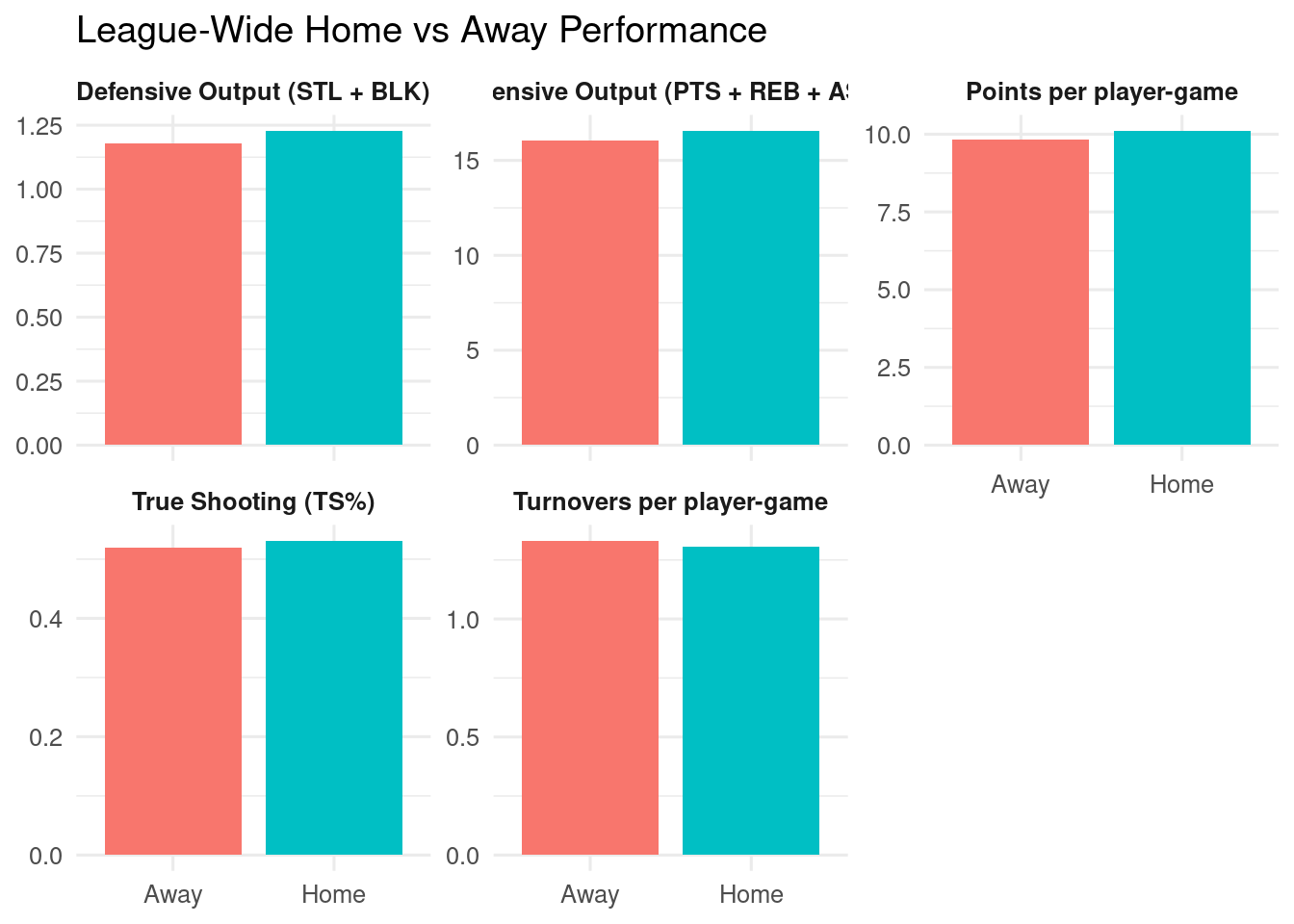
# Let's add some composite measures of offensive and defensive stat creation. 
pb <- pb %>%
  filter(!did_not_play, minutes > 0) %>%
  mutate(
    # True Shooting Percentage
    denom = 2 * (field_goals_attempted + 0.44 * free_throws_attempted),
    ts = if_else(denom > 0, points / denom, NA_real_),

    # Composite performance metrics
    offensive_output = points + rebounds + assists,
    defensive_output = steals + blocks
  )

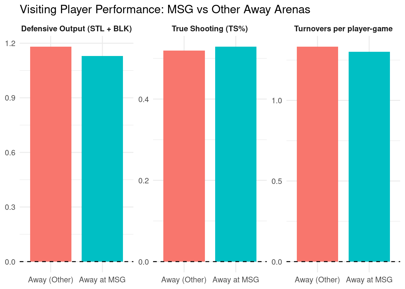
# Create dataset of all player box scores only from games at MSG. Categorize home/away players. Calculate TS%. 
pb_msg <- pb %>%
  inner_join(
    msg_knicks_home_games,
    by = c("game_id", "season", "season_type", "game_date")
  ) %>%
  mutate(
    at_msg = TRUE,
    is_knicks = (team_abbreviation == "NY"),
    is_home = (home_away == "home"),
    is_away = (home_away == "away"),
    ts = points / (2 * (field_goals_attempted + 0.44 * free_throws_attempted))
  )

pb_road_flagged <- pb %>%
  filter(home_away == "away", !did_not_play, minutes > 0) %>%
  left_join(
    msg_knicks_home_games %>% transmute(game_id, at_msg = TRUE),
    by = "game_id"
  ) %>%
  mutate(
    at_msg = if_else(is.na(at_msg), FALSE, at_msg),
    ts = points / (2 * (field_goals_attempted + 0.44 * free_throws_attempted))
  )

4.4 —————————————————————————–

4.5 Q1: Do the New York Knicks experience a special home-court advantage due to playing at MSG?

4.5.0.1 Where do the Knicks rank in terms of home court advantage?

Show the code
# Let's find each team's home court advantage (average total points scored at home - average total points scored away). 

non_nba_teams <- c("EAST", "WEST", "USA", "WORLD", "GIA", "LEB")

team_game <- pb %>%
  filter(
    !did_not_play,
    minutes > 0,
  ) %>%
  group_by(game_id, team_abbreviation, home_away) %>%
  summarise(
    team_points = sum(points, na.rm = TRUE),
    .groups = "drop"
  )

team_home_away <- team_game %>%
  filter(!team_abbreviation %in% non_nba_teams) %>%
  group_by(team_abbreviation, home_away) %>%
  summarise(
    avg_points = mean(team_points, na.rm = TRUE),
    .groups = "drop"
  )
team_home_advantage <- team_home_away %>%
  pivot_wider(
    names_from = home_away,
    values_from = avg_points
  ) %>%
  mutate(
    home_court_advantage = home - away
  ) %>%
  select(team_abbreviation, home_court_advantage)

nba_abbrevs <- sched %>%
  select(home_abbreviation, away_abbreviation) %>%
  pivot_longer(
    cols = everything(),
    values_to = "team_abbreviation"
  ) %>%
  distinct(team_abbreviation)

team_home_advantage_nba <- team_home_advantage %>%
  semi_join(nba_abbrevs, by = "team_abbreviation")

knicks_abbrevs <- c("NY", "NYK")

team_home_advantage_ranked <- team_home_advantage_nba %>%
  mutate(is_knicks = team_abbreviation %in% knicks_abbrevs) %>%
  arrange(desc(home_court_advantage)) %>%
  mutate(rank = row_number())

# Display: 
knicks_row <- team_home_advantage_ranked %>%
  filter(is_knicks)

display_table <- team_home_advantage_ranked %>%
  filter(!team_abbreviation %in% non_nba_teams) %>%
  mutate(
    home_court_advantage = round(home_court_advantage, 2)
  ) %>%
  select(rank, team_abbreviation, home_court_advantage)

knitr::kable(
  display_table,
  caption = "Team-Level Home Court Advantage (Home − Away Points)"
)
Table 4.1: Team-Level Home Court Advantage (Home − Away Points)
rank team_abbreviation home_court_advantage
1 POR 4.44
2 DEN 4.35
3 ATL 3.74
4 WSH 3.66
5 MIL 3.61
6 SAC 3.60
7 GS 3.57
8 MIA 3.46
9 OKC 3.40
10 SA 3.39
11 IND 3.34
12 UTAH 3.28
13 NJ 3.16
14 DAL 3.05
15 CLE 3.01
16 NO 2.98
17 ORL 2.93
18 MEM 2.76
19 TOR 2.75
20 DET 2.61
21 LAL 2.48
22 PHX 2.46
23 NY 2.43
24 PHI 2.25
25 CHA 2.23
26 BOS 2.12
27 SEA 2.04
28 LAC 1.97
29 HOU 1.54
30 CHI 0.89
31 MIN 0.85
32 BKN 0.74

4.5.0.2 New York’s home court advantage ranks 23rd on the list of NBA teams, placing them in the bottom third of the league. However, their home–away scoring differential was close to the league average, indicating that Madison Square Garden does not confer a markedly weaker or stronger team-level advantage.

4.6 —————————————————————————–

4.7 Q2: Do visiting players play differently at MSG than other arenas?

4.7.1 For context, let’s look at the league-wide home vs. away comparisons.

Show the code
league_home_away <- pb %>%
  filter(!did_not_play, minutes > 0) %>%
  mutate(
    location = if_else(home_away == "home", "Home", "Away"),
    ts = points / (2 * (field_goals_attempted + 0.44 * free_throws_attempted))
  ) %>%
  group_by(location) %>%
  summarise(
    games = n_distinct(game_id),
    pts = mean(points, na.rm = TRUE),
    ts  = mean(ts, na.rm = TRUE),
    tov = mean(turnovers, na.rm = TRUE),
    offensive_output = mean(offensive_output, na.rm = TRUE),
    defensive_output = mean(defensive_output, na.rm = TRUE),
    .groups = "drop"
  )

kable(league_home_away, caption = "League-wide home vs. away player averages across key performance metrics (2002–present).")
Table 4.2: League-wide home vs. away player averages across key performance metrics (2002–present).
location games pts ts tov offensive_output defensive_output
Away 31510 9.843075 0.5195918 1.332021 16.05069 1.179258
Home 31510 10.114903 0.5314177 1.304944 16.56729 1.228689
Show the code
t.test(points ~ home_away, data = pb)

    Welch Two Sample t-test

data:  points by home_away
t = -13.213, df = 651914, p-value < 2.2e-16
alternative hypothesis: true difference in means between group away and group home is not equal to 0
95 percent confidence interval:
 -0.3121486 -0.2315065
sample estimates:
mean in group away mean in group home 
          9.843075          10.114903 
Show the code
# Players score more points (+0.27 PTS/G) at home vs. away (p-value < .001). 
t.test(ts ~ home_away, data = pb)

    Welch Two Sample t-test

data:  ts by home_away
t = -18.298, df = 624686, p-value < 2.2e-16
alternative hypothesis: true difference in means between group away and group home is not equal to 0
95 percent confidence interval:
 -0.01309258 -0.01055920
sample estimates:
mean in group away mean in group home 
         0.5195918          0.5314177 
Show the code
# Players score more efficiently (+1.19 TS%) at home vs. away (p-value < .001).
t.test(turnovers ~ home_away, data = pb)

    Welch Two Sample t-test

data:  turnovers by home_away
t = 7.7703, df = 651902, p-value = 7.839e-15
alternative hypothesis: true difference in means between group away and group home is not equal to 0
95 percent confidence interval:
 0.02024722 0.03390688
sample estimates:
mean in group away mean in group home 
          1.332021           1.304943 
Show the code
# Players turn the ball over less often (-0.03 TO/G) at home vs. away (p-value < .001).
t.test(offensive_output ~ home_away, data = pb)

    Welch Two Sample t-test

data:  offensive_output by home_away
t = -17.932, df = 651761, p-value < 2.2e-16
alternative hypothesis: true difference in means between group away and group home is not equal to 0
95 percent confidence interval:
 -0.5730664 -0.4601348
sample estimates:
mean in group away mean in group home 
          16.05069           16.56729 
Show the code
# Players produce more offensive stats (+0.52) at home vs. away (p-value < .001). 
t.test(defensive_output ~ home_away, data = pb)

    Welch Two Sample t-test

data:  defensive_output by home_away
t = -14.772, df = 651194, p-value < 2.2e-16
alternative hypothesis: true difference in means between group away and group home is not equal to 0
95 percent confidence interval:
 -0.05598975 -0.04287250
sample estimates:
mean in group away mean in group home 
          1.179258           1.228689 
Show the code
# Players produce more defensive stats (+0.05) at home vs. away (p-value < .001).


league_long <- league_home_away %>%
  pivot_longer(
    cols = c(pts, ts, tov, offensive_output, defensive_output),
    names_to = "metric",
    values_to = "value"
  ) %>%
  mutate(
    metric = recode(metric,
      pts = "Points per player-game",
      ts  = "True Shooting (TS%)",
      tov = "Turnovers per player-game",
      offensive_output = "Offensive Output (PTS + REB + AST)",
      defensive_output = "Defensive Output (STL + BLK)"
    )
  )

league_long <- league_long %>%
  group_by(metric) %>%
  mutate(z_value = (value - mean(value)) / sd(value)) %>%
  ungroup()
Show the code
# Bar plot 
ggplot(league_long, aes(x = location, y = value, fill = location)) +
  geom_col(width = .85) +
  facet_wrap(~ metric, scales = "free_y") +
  labs(
    title = "League-Wide Home vs Away Performance",
    x = NULL,
    y = NULL
  ) +
  theme_minimal(base_size = 12) +
  theme(
    legend.position = "none",
    strip.text = element_text(face = "bold")
  )
Facet bar chart comparing Home vs Away averages for points, true shooting percentage, turnovers, offensive output, and defensive output. Home is higher for points, true shooting, offensive output, and defensive output, and lower for turnovers.
Figure 4.1: League-wide comparison of average player performance in home vs away games across five metrics.

4.7.1.1 Across the league, players perform better at home games than away games.

4.7.2 Let’s see if visiting players play better or worse at MSG compared to other away games.

Show the code
# Do visiting players post better or worse averages at MSG compared to other arenas?

# Note: To isolate the effect of Madison Square Garden on visiting teams, analyses were restricted to away games only. As a result, all Knicks home games were excluded, and MSG performances reflect exclusively visiting team data.
opponent_msg_summary <- pb_road_flagged %>%
  group_by(at_msg) %>%
  summarise(
    games = n_distinct(game_id),
    pts = mean(points, na.rm = TRUE),
    ts  = mean(ts, na.rm = TRUE),
    tov = mean(turnovers, na.rm = TRUE),
    offensive_output = mean(offensive_output, na.rm = TRUE),
    defensive_output = mean(defensive_output, na.rm = TRUE),
    .groups = "drop"
  )
opponent_msg_summary
# A tibble: 2 × 7
  at_msg games   pts    ts   tov offensive_output defensive_output
  <lgl>  <int> <dbl> <dbl> <dbl>            <dbl>            <dbl>
1 FALSE  30526  9.84 0.519  1.33             16.1             1.18
2 TRUE     984  9.95 0.529  1.30             16.1             1.13
Show the code
t.test(points ~ at_msg, data = pb_road_flagged)

    Welch Two Sample t-test

data:  points by at_msg
t = -1.3646, df = 10811, p-value = 0.1724
alternative hypothesis: true difference in means between group FALSE and group TRUE is not equal to 0
95 percent confidence interval:
 -0.28143672  0.05041087
sample estimates:
mean in group FALSE  mean in group TRUE 
           9.839470            9.954983 
Show the code
# The difference in scoring (+0.12 PTS/G) by visiting players at MSG compared to other arenas is not statistically significant (p-value = 0.14). 

t.test(ts ~ at_msg, data = pb_road_flagged)

    Welch Two Sample t-test

data:  ts by at_msg
t = -3.6045, df = 10346, p-value = 0.0003142
alternative hypothesis: true difference in means between group FALSE and group TRUE is not equal to 0
95 percent confidence interval:
 -0.014793219 -0.004371289
sample estimates:
mean in group FALSE  mean in group TRUE 
          0.5192936           0.5288758 
Show the code
# The difference in shooting efficiency (+1.0 TS%) at MSG compared to other arenas *is* statistically significant (p-value < .001).

t.test(turnovers ~ at_msg, data = pb_road_flagged)

    Welch Two Sample t-test

data:  turnovers by at_msg
t = 2.2578, df = 10862, p-value = 0.02398
alternative hypothesis: true difference in means between group FALSE and group TRUE is not equal to 0
95 percent confidence interval:
 0.004185506 0.059321161
sample estimates:
mean in group FALSE  mean in group TRUE 
           1.333011            1.301258 
Show the code
# The difference in turnovers committed (-0.03 TO/G) at MSG compared to other arenas *is* statistically significant (p-value = .029).

t.test(offensive_output ~ at_msg, data = pb_road_flagged)

    Welch Two Sample t-test

data:  offensive_output by at_msg
t = -0.088159, df = 10816, p-value = 0.9298
alternative hypothesis: true difference in means between group FALSE and group TRUE is not equal to 0
95 percent confidence interval:
 -0.2411585  0.2203999
sample estimates:
mean in group FALSE  mean in group TRUE 
           16.05036            16.06074 
Show the code
# The difference in offensive stat creation (+0.10) is not statistically significant (p-value = 0.87).

t.test(defensive_output ~ at_msg, data = pb_road_flagged)

    Welch Two Sample t-test

data:  defensive_output by at_msg
t = 3.8684, df = 10875, p-value = 0.0001102
alternative hypothesis: true difference in means between group FALSE and group TRUE is not equal to 0
95 percent confidence interval:
 0.02486178 0.07593904
sample estimates:
mean in group FALSE  mean in group TRUE 
           1.180831            1.130431 
Show the code
# The difference in defensive stat creation (+0.05) *is* statistically significant (p-value < .001).

road_means <- pb_road_flagged %>%
  group_by(at_msg) %>%
  summarise(
    ts = mean(ts, na.rm = TRUE),
    turnovers = mean(turnovers, na.rm = TRUE),
    defensive_output = mean(defensive_output, na.rm = TRUE),
    .groups = "drop"
  ) %>%
  mutate(
    location = if_else(at_msg, "Away at MSG", "Away (Other)")
  ) %>%
  select(location, ts, turnovers, defensive_output)

road_long <- road_means %>%
  pivot_longer(
    cols = c(ts, turnovers, defensive_output),
    names_to = "metric",
    values_to = "value"
  ) %>%
  mutate(
    metric = recode(metric,
      ts = "True Shooting (TS%)",
      turnovers = "Turnovers per player-game",
      defensive_output = "Defensive Output (STL + BLK)"
    ),
    location = factor(location, levels = c("Away (Other)", "Away at MSG"))
  )
Show the code
ggplot(road_long, aes(x = location, y = value, fill = location)) +
  geom_col(width = 0.8) +
  theme(axis.text.x = element_text(angle = 45, hjust = 1, vjust = 1)) +
  facet_wrap(~ metric, scales = "free_y") +
  geom_hline(yintercept = 0, linetype = "dashed") +
  labs(
    title = "Visiting Player Performance: MSG vs Other Away Arenas",
    x = NULL,
    y = NULL
  ) +
  theme_minimal(base_size = 12) +
  theme(
    legend.position = "none",
    strip.text = element_text(face = "bold")
  )
Facet bar chart comparing Away at MSG vs Away (Other). Away at MSG shows slightly higher true shooting, slightly fewer turnovers, and slightly higher defensive output.
Figure 4.2: Visiting player averages at Madison Square Garden compared with other away arenas for true shooting, turnovers, and defensive output.

4.7.2.1 Compared to other away games, players shoot more efficiently, turn the ball over less often, and produce more defensive stats when they play away games at MSG. This supports the notion that playing at MSG may elevate performances more than playing at other stadiums, at least for visiting players. This leads us to our next question.

4.8 —————————————————————————–

4.9 Q3: Who benefits the most from playing at MSG?

4.9.1 Which players put up the best performances at MSG? (min = 8 games played at MSG)

WarningImportant note about the data

The figures below use data from away games played at Madison Square Garden (MSG).
Because Knicks players do not play away games at MSG, their “MSG” data reflects games they played at MSG as members of other teams, not as Knicks.

Show the code
player_msg_overall <- pb_road_flagged %>%
  filter(at_msg == TRUE, !did_not_play, minutes >= 15) %>%
  mutate(
    total_output = offensive_output + defensive_output
  ) %>%
  group_by(athlete_id, athlete_display_name) %>%
  summarise(
    games   = n(),
    avg_pts = mean(points, na.rm = TRUE),
    avg_ts  = mean(ts, na.rm = TRUE),
    avg_off = mean(offensive_output, na.rm = TRUE),
    avg_def = mean(defensive_output, na.rm = TRUE),
    avg_tot = mean(total_output, na.rm = TRUE),
    .groups = "drop"
  )


player_msg_overall_clean <- player_msg_overall %>%
  filter(games >= 8)

# Here are the top 20 players with the highest total outputs at MSG. 
player_msg_overall_clean %>%
  arrange(desc(avg_tot)) %>%
  select(
    athlete_display_name,
    games,
    avg_pts,
    avg_ts,
    avg_off,
    avg_def,
    avg_tot
  ) %>%
  head(20)
# A tibble: 20 × 7
   athlete_display_name  games avg_pts avg_ts avg_off avg_def avg_tot
   <chr>                 <int>   <dbl>  <dbl>   <dbl>   <dbl>   <dbl>
 1 Kobe Bryant              12    33.9  0.623    44.1    1.83    45.9
 2 Anthony Davis             9    28.6  0.602    42.6    3       45.6
 3 LeBron James             32    28.0  0.591    42.4    2.53    45.0
 4 Kevin Durant             11    31.2  0.659    43.4    1.55    44.9
 5 James Harden             15    27.3  0.629    41.7    2.6     44.3
 6 Joel Embiid              11    27.5  0.595    41.4    2.27    43.6
 7 Giannis Antetokounmpo    20    23.4  0.593    40.0    2.5     42.4
 8 Stephen Curry            12    28.3  0.623    39.9    1.83    41.8
 9 Allen Iverson            12    26.6  0.469    38.1    2.5     40.6
10 Nikola Jokic             11    24    0.639    39.4    1.09    40.5
11 Russell Westbrook        18    21.7  0.521    38.2    1.89    40.1
12 Trae Young               11    25.6  0.529    38.4    1.18    39.5
13 Devin Booker             10    30.8  0.607    37.6    1.3     38.9
14 Donovan Mitchell         11    26.6  0.577    36.5    1.82    38.3
15 Dirk Nowitzki            15    26.5  0.636    36.5    1.47    38  
16 Jayson Tatum             14    23.6  0.572    35.1    2.57    37.6
17 DeMarcus Cousins          9    20.2  0.528    34.3    3.22    37.6
18 Zach LaVine              10    26.8  0.615    35.5    1.7     37.2
19 Kyrie Irving             12    26    0.593    35.9    1.25    37.2
20 Tracy McGrady            11    23.1  0.516    34.1    2.27    36.4
Show the code
# Here are the top 20 players with the highest true shooting % at MSG. 
player_msg_overall_clean %>%
  arrange(desc(avg_ts)) %>%
  select(
    athlete_display_name,
    games,
    avg_pts,
    avg_ts,
    avg_off,
    avg_def
  ) %>%
  head(20)
# A tibble: 20 × 6
   athlete_display_name games avg_pts avg_ts avg_off avg_def
   <chr>                <int>   <dbl>  <dbl>   <dbl>   <dbl>
 1 Joe Ingles               8   10.6   0.774    17.1   0.625
 2 Patrick Patterson       10    8.5   0.772    13.3   1.6  
 3 DeAndre Jordan          12   11.1   0.749    21.7   2.08 
 4 Rudy Gobert             11   12.4   0.739    22.5   2.27 
 5 Kevin Martin             8   24.2   0.712    30     1.38 
 6 Dwight Powell            8    6.25  0.710    11.9   0.625
 7 Jae Crowder             11   14.1   0.690    19.4   1.09 
 8 Jonas Jerebko           10    8.5   0.685    14.7   1    
 9 Wally Szczerbiak         9   16.4   0.684    22.7   1    
10 Richaun Holmes           8   10.2   0.682    16.9   1.5  
11 Joe Harris               9    9.67  0.682    13.7   0.667
12 Nick Collison            8    6.88  0.680    12.8   0.875
13 Blake Griffin           10   21     0.676    30.7   1.6  
14 Cameron Johnson          8   16.2   0.674    21.5   0.75 
15 Kelly Olynyk            14   10.6   0.671    16.8   0.786
16 JJ Redick               15   16     0.666    20.4   0.333
17 Ed Davis                 9    9.67  0.665    17.8   1    
18 Draymond Green          12   10.6   0.664    23.8   2.92 
19 Tim Hardaway Jr.        10   15.8   0.661    20.9   0.9  
20 Corey Maggette          10   18.9   0.661    25     0.9  

4.9.2 Who steps up their game the most playing at MSG vs. other away games?

Show the code
# Let's compute every player's MSG advantage score = (average offensive + defensive output at MSG away games - average offensive + defensive output at other away games). 
player_msg_advantage <- pb_road_flagged %>%
  filter(!did_not_play, minutes >= 15) %>%
  mutate(total_output = offensive_output + defensive_output) %>%
  group_by(athlete_id, athlete_display_name, at_msg) %>%
  summarise(
    games = n(),
    avg_total = mean(total_output, na.rm = TRUE),
    avg_pts   = mean(points, na.rm = TRUE),
    avg_ts    = mean(ts, na.rm = TRUE),
    .groups = "drop"
  ) %>%
  pivot_wider(
    names_from = at_msg,
    values_from = c(games, avg_total, avg_pts, avg_ts)
  ) %>%
  mutate(
    msg_adv_total = avg_total_TRUE - avg_total_FALSE,
    msg_adv_pts   = avg_pts_TRUE   - avg_pts_FALSE,
    msg_adv_ts    = avg_ts_TRUE    - avg_ts_FALSE
  ) 

player_msg_advantage <- player_msg_advantage %>%
  filter(games_TRUE >= 8)

# Let's identify the top MSG risers and chokers. 

msg_extremes <- bind_rows(
  player_msg_advantage %>% arrange(desc(msg_adv_total)) %>% slice_head(n = 20) %>% mutate(group = "MSG Risers"),
  player_msg_advantage %>% arrange(msg_adv_total)       %>% slice_head(n = 20) %>% mutate(group = "MSG Chokers")
) %>%
  mutate(
    athlete_display_name = factor(athlete_display_name, levels = athlete_display_name[order(msg_adv_total)])
  )

msg_extremes <- msg_extremes
Show the code
ggplot(msg_extremes, aes(x = msg_adv_total, y = athlete_display_name, fill = group)) +
  geom_col(width = 0.75) +
  facet_wrap(~ group, scales = "free_y") +
  geom_vline(xintercept = 0, linetype = "dashed", color = "grey40") +
  labs(
    title = "MSG Risers and Chokers: Total Stat Output",
    subtitle = "Within-player difference in total output at MSG vs other away games",
    x = "MSG Total Output − Other Away Total Output",
    y = NULL
  ) +
  theme_minimal(base_size = 12) +
  theme(legend.position = "none", strip.text = element_text(face = "bold"))
Two-panel horizontal bar chart. Left panel shows players with the largest positive change in total output at MSG compared with other away games; right panel shows the largest negative change. Bars represent within-player differences.
Figure 4.3: Players whose total stat output changes most at MSG versus other away games, shown as top ‘riser’ and ‘choker’ differences.

4.9.2.1 These are the players whose statistical outputs change the most playing at MSG vs. other arenas. Knicks fans, do any stand out in your memory? Do any surprise you?

4.9.3 Let’s also look at shooting efficiency.

Show the code
ts_extremes <- bind_rows(
  player_msg_advantage %>% arrange(desc(msg_adv_ts)) %>% slice_head(n = 20) %>% mutate(group = "TS Risers"),
  player_msg_advantage %>% arrange(msg_adv_ts)       %>% slice_head(n = 20) %>% mutate(group = "TS Chokers")
) %>%
  mutate(
    athlete_display_name = factor(athlete_display_name, levels = athlete_display_name[order(msg_adv_ts)])
  )
Show the code
ggplot(ts_extremes, aes(x = msg_adv_ts, y = athlete_display_name, fill = group)) +
  geom_col(width = 0.75) +
  facet_wrap(~ group, scales = "free_y") +
  geom_vline(xintercept = 0, linetype = "dashed", color = "grey40") +
  labs(
    title = "MSG Risers and Chokers: Shooting Efficiency",
    subtitle = "Within-player difference in True Shooting at MSG vs other away games",
    x = "MSG Advantage (TS%)",
    y = NULL
  ) +
  theme_minimal(base_size = 12) +
  theme(legend.position = "none", strip.text = element_text(face = "bold"))
Two-panel horizontal bar chart. One panel shows players with the largest increases in true shooting at MSG; the other shows the largest decreases. Bars represent within-player differences in TS% at MSG versus other away games.
Figure 4.4: Players whose true shooting percentage changes most at MSG versus other away games.

4.9.3.1 These are the players whose shooting efficiency changed the most playing at MSG vs. other arenas.

4.9.4 How do the stars of the NBA today perform at MSG compared to other venues?

Show the code
# Let's make a dataset using recent all-stars from 2024 and 2025. 
recent_all_stars <- c(
  "LeBron James", "Stephen Curry", "Kevin Durant", "Giannis Antetokounmpo",
  "Nikola Jokic", "Joel Embiid", "Luka Doncic", "Jayson Tatum",
  "Jimmy Butler", "Damian Lillard", "Anthony Davis", "Kawhi Leonard",
  "Shai Gilgeous-Alexander", "Devin Booker", "Jaylen Brown", "Kyrie Irving",
  "Tyrese Haliburton", "Donovan Mitchell", "Bam Adebayo", "Jalen Brunson",
  "Anthony Edwards", "Julius Randle", "Trae Young", "Pascal Siakam", 
  "James Harden", "Jalen Williams", "Evan Mobley", "Victor Wembanyama",
  "Cade Cunningham", "Tyler Herro", "Jaren Jackson Jr.", "Darius Garland",
  "Alperen Sengun", "Tyrese Maxey", "Paolo Banchero", "Scottie Barnes"
)

# Remove the MSG game minimum for the young guys on this list. (This is ugly but I figured it'd work)
player_msg_advantage1 <- pb_road_flagged %>%
  filter(!did_not_play, minutes >= 15) %>%
  mutate(total_output = offensive_output + defensive_output) %>%
  group_by(athlete_id, athlete_display_name, at_msg) %>%
  summarise(
    games = n(),
    avg_total = mean(total_output, na.rm = TRUE),
    avg_pts   = mean(points, na.rm = TRUE),
    avg_ts    = mean(ts, na.rm = TRUE),
    .groups = "drop"
  ) %>%
  pivot_wider(
    names_from = at_msg,
    values_from = c(games, avg_total, avg_pts, avg_ts)
  ) %>%
  mutate(
    msg_adv_total = avg_total_TRUE - avg_total_FALSE,
    msg_adv_pts   = avg_pts_TRUE   - avg_pts_FALSE,
    msg_adv_ts    = avg_ts_TRUE    - avg_ts_FALSE
  ) 

allstar_msg_adv <- player_msg_advantage1 %>%
  filter(athlete_display_name %in% recent_all_stars) %>%
  mutate(
    msg_adv_ts = msg_adv_ts * 100)
Show the code
# Let's make a scatterplot with TS% change on the y axis, offensive output change on the x axis. 
library(ggrepel)
Warning: package 'ggrepel' was built under R version 4.5.2
Show the code
ggplot(player_msg_advantage1,
       aes(x = msg_adv_total, y = msg_adv_ts)) +
  geom_point(
    data = allstar_msg_adv,
    size = 3,
  ) +

  geom_text_repel(
    data = allstar_msg_adv,
    aes(label = athlete_display_name),
    size = 3,
    color = "blue",
    max.overlaps = Inf
  ) +

  geom_hline(yintercept = 0, linetype = "dashed", color = "grey50") +
  geom_vline(xintercept = 0, linetype = "dashed", color = "grey50") +

  labs(
    title = "How Recent NBA All-Stars Perform at Madison Square Garden",
    subtitle = "Differences in offensive output (x) and shooting efficiency (y) at MSG",
    x = "Change in Total Stat (Offensive + Defensive) Output",
    y = "Change in TS percentage points"
  ) +
  theme_minimal(base_size = 12) 
Scatter plot of selected All-Stars, with x-axis as change in total output at MSG versus other away games and y-axis as change in true shooting percentage. Points are labeled by player name; quadrants indicate better or worse output and efficiency at MSG.
Figure 4.5: Recent NBA All-Stars: change in total output and change in true shooting at MSG versus other away games.

4.9.4.1 Durant, Harden, Cunningham, and other players in the top right quadrant play better overall at MSG compared to other away games. Butler, Haliburton, Sengun, and other players in the bottom left quadrant perform worse overall. Wembanyama and other players in the bottom right quadrant produce more stats but do so less efficiently at MSG.

4.9.4.2 Brunson and Randle’s games as Knicks players were not included in these analyses.

4.10 —————————————————————————–

4.11 Conclusion: Is the MSG Effect detectable?

4.11.1 On an individual player performance level: yes.

4.11.1.1 Our analyses from Q2 showed that visiting players shot more efficiently, turned the ball over less, and produced more defensive stats on average playing at MSG compared to other away games. This supports the notion that visiting players may be more “locked in” on average for games at The Garden. Analyses from Q3 answered who rose to the occasion vs. who choked under the pressure of The Garden. Some players consistently performed better at MSG, while others performed worse. These are the players who seem to be most influenced by the MSG Effect, positively and negatively.

4.11.1.2 Overall, these findings suggest that Madison Square Garden functions less as a traditional home court advantage and more as a high-visibility performance context that accentuates player-specific responses to pressure, attention, and atmosphere.