5 Final Project

Author

Isley Jean-Pierre

6 Final Project

This is a project that I hope to present at the NYC OpenData conference next spring. I must admit that there are some datasets that I intended to use for this final assignment, but because of time and roadblocks, I will focus on the two keys datasets for now. My goal is to keep on this project by finding a meaningful way to include the other datasets. I believe that this project has the potential to become something special.

Show the code

library(tidyverse)

Warning: package 'tidyr' was built under R version 4.5.2

Warning: package 'readr' was built under R version 4.5.2

Warning: package 'purrr' was built under R version 4.5.2

── Attaching core tidyverse packages ──────────────────────── tidyverse 2.0.0 ──
✔ dplyr     1.1.4     ✔ readr     2.1.5
✔ forcats   1.0.1     ✔ stringr   1.6.0
✔ ggplot2   4.0.0     ✔ tibble    3.3.0
✔ lubridate 1.9.4     ✔ tidyr     1.3.1
✔ purrr     1.2.0     
── Conflicts ────────────────────────────────────────── tidyverse_conflicts() ──
✖ dplyr::filter() masks stats::filter()
✖ dplyr::lag()    masks stats::lag()
ℹ Use the conflicted package (<http://conflicted.r-lib.org/>) to force all conflicts to become errors

Show the code

library(dplyr)
library(Hmisc)

Warning: package 'Hmisc' was built under R version 4.5.2


Attaching package: 'Hmisc'

The following objects are masked from 'package:dplyr':

    src, summarize

The following objects are masked from 'package:base':

    format.pval, units

Show the code

library(ggplot2)
library(corrplot)

corrplot 0.95 loaded

Show the code

library(lubridate)
library(nycOpenData)

6.1 Let’s load the dataset

Show the code

rea <- nycOpenData::nyc_dop_juvenile_rearrest_rate(limit= 10000)
head(rea)

# A tibble: 6 × 4
  borough  month     year  rate 
  <chr>    <chr>     <chr> <chr>
1 Citywide September 2025  4.5  
2 Citywide December  2025  4.4  
3 Citywide July      2025  5.3  
4 Citywide October   2025  4.4  
5 Citywide August    2025  4.6  
6 Citywide November  2025  4.5

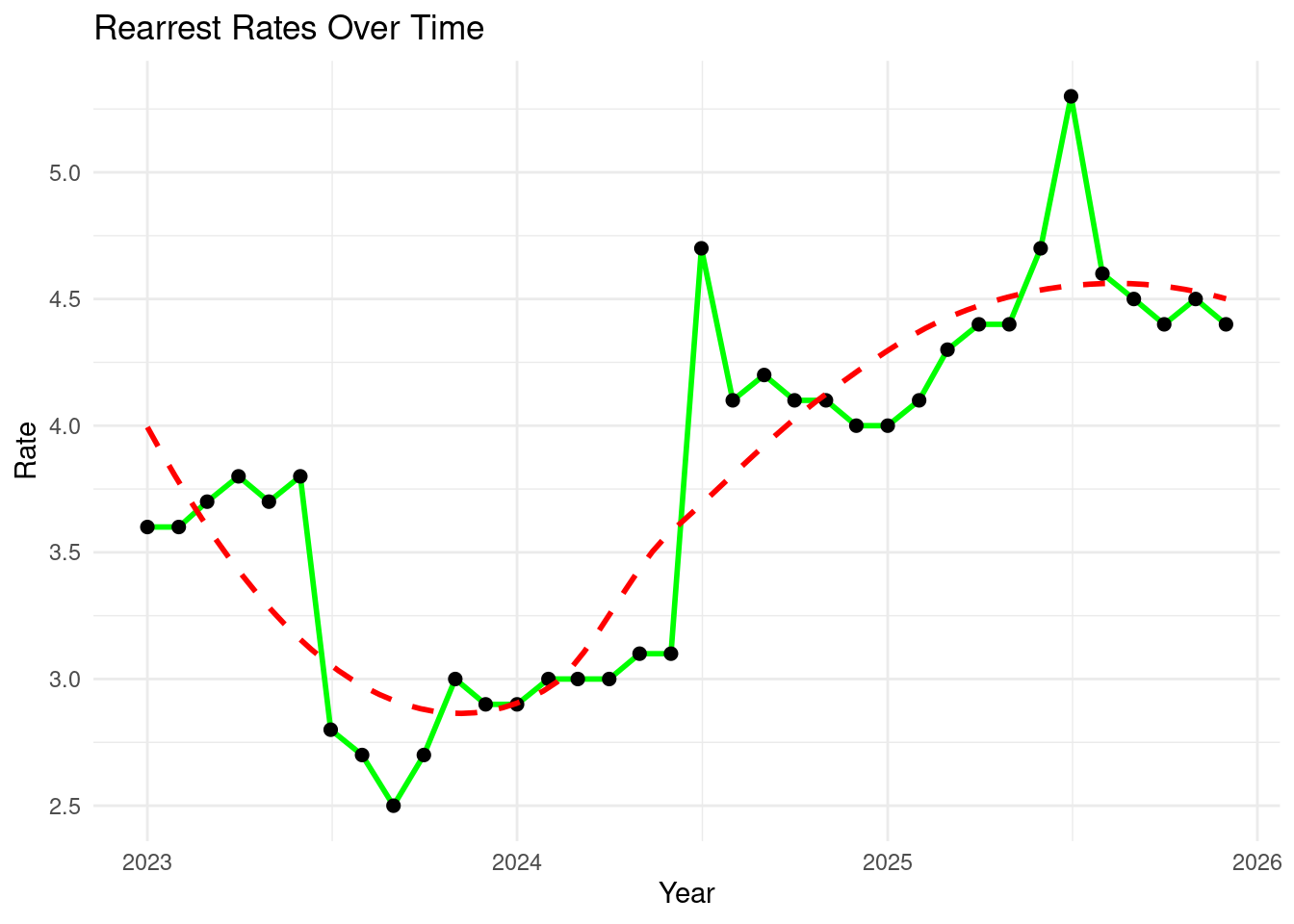
6.2 Let’s focus on the years between 2023 and 2025

Show the code

rea_clean <- rea %>%
  filter(year >= 2023 & year <= 2025)
head(rea_clean)

# A tibble: 6 × 4
  borough  month     year  rate 
  <chr>    <chr>     <chr> <chr>
1 Citywide September 2025  4.5  
2 Citywide December  2025  4.4  
3 Citywide July      2025  5.3  
4 Citywide October   2025  4.4  
5 Citywide August    2025  4.6  
6 Citywide November  2025  4.5

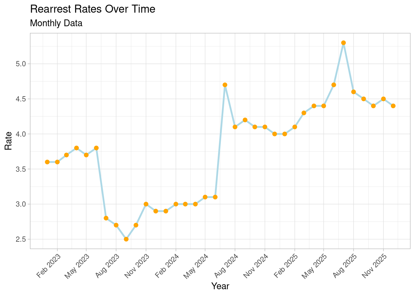
6.3 Let’s create a new column that contains month and year

Show the code

rea_clean <- rea_clean %>%
  mutate(
    month_year = paste(month,year, sep = " "),
    month_year = my(month_year)
  )

6.4 Removing the previous columns

Show the code

rea_clean <- rea_clean %>%
  select(-month, -year)

6.5 Let’s see if we can find a correlation between rearrest rates and date Before that let’s make sure that the columns are in the right format

Show the code

str(rea_clean)

tibble [36 × 3] (S3: tbl_df/tbl/data.frame)
 $ borough   : chr [1:36] "Citywide" "Citywide" "Citywide" "Citywide" ...
 $ rate      : chr [1:36] "4.5" "4.4" "5.3" "4.4" ...
 $ month_year: Date[1:36], format: "2025-09-01" "2025-12-01" ...

To see the structure.

Show the code

rea_clean <- rea_clean %>%
  mutate(
    rate = as.numeric(rate)  # Making rate into numeric instead of character
  )

6.6 Let’s look at the sum of rearrest rates per year

Show the code

sum_year <- rea_clean %>%
  mutate(year = year(month_year)) %>%
  group_by(year) %>%
  summarise(
    total_rate = sum(rate, na.rm = TRUE)
  )
sum_year

# A tibble: 3 × 2
   year total_rate
  <dbl>      <dbl>
1  2023       38.8
2  2024       43.3
3  2025       53.6

6.7 For fun, let’s look at the average rearrest rates per year

Show the code

avg_rea_year <- rea_clean %>%
  mutate(year = year(month_year)) %>%
  group_by(year) %>%
  summarise(
    mean_rate = mean(rate, na.rm = TRUE)
  )
avg_rea_year

# A tibble: 3 × 2
   year mean_rate
  <dbl>     <dbl>
1  2023      3.23
2  2024      3.61
3  2025      4.47

6.8 Investigating the months

Let’s take a closer look to see if there are some months where rearrest rates are higher than others

Show the code

month_repeat <- rea_clean %>%
  mutate(month = month(month_year, label = TRUE)) %>%
  group_by(month) %>%
  summarise(
    mean_rate = mean(rate, na.rm = TRUE)
  )
month_repeat

# A tibble: 12 × 2
   month mean_rate
   <ord>     <dbl>
 1 Jan        3.5 
 2 Feb        3.57
 3 Mar        3.67
 4 Apr        3.73
 5 May        3.73
 6 Jun        3.87
 7 Jul        4.27
 8 Aug        3.8 
 9 Sep        3.73
10 Oct        3.73
11 Nov        3.87
12 Dec        3.77

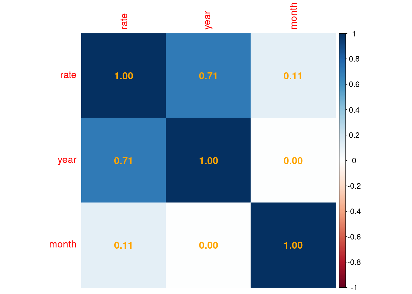
6.9 Let’s finally see if we can find a correlation between rearrest rates and year

Show the code

cor(as.numeric(rea_clean$rate), as.numeric(rea_clean$month_year))

[1] 0.7071394

It seems that there is indeed a strong correlation between rearrest rates and year with r = 0.69.

6.10 Trying to run a correlation Matrix

Show the code

rea_cor <- rea_clean %>%
  mutate(
    year         = lubridate::year(month_year),
    month        = lubridate::month(month_year)
  ) %>%
  select(rate, year, month)

Show the code

cor_matrix <- cor(rea_cor)
cor_matrix

           rate      year     month
rate  1.0000000 0.7097743 0.1139991
year  0.7097743 1.0000000 0.0000000
month 0.1139991 0.0000000 1.0000000

6.11 Building the Correlation Matrix

Show the code

corrplot(cor_matrix, method = "color", addCoef.col = "orange")

6.12 Playing with ggplot

Show the code

ggplot(rea_clean, aes(x = month_year, y = rate)) +
  geom_line(color = "green", size = 1) +
  geom_point(color = "black", size = 2) +
  geom_smooth(method = "loess", se = FALSE, color = "red", linetype = "dashed") +
  labs(
    title = "Rearrest Rates Over Time",
    x = "Year",
    y = "Rate"
  ) +
  theme_minimal()

Warning: Using `size` aesthetic for lines was deprecated in ggplot2 3.4.0.
ℹ Please use `linewidth` instead.

`geom_smooth()` using formula = 'y ~ x'

This figure shows rearrest rates over time.

6.13 Playing with ggplot (adding months into the graph)

Show the code

ggplot(rea_clean, aes(x = month_year, y = rate)) +
  geom_line(color = "lightblue", size = 1) +
  geom_point(color = "orange", size = 2) +
  labs(
    title = "Rearrest Rates Over Time",
    subtitle = "Monthly Data",
    x = "Year",
    y = "Rate"
  ) +
  scale_x_date(date_breaks = "3 months", date_labels = "%b %Y") +
  theme_light() +
  theme(axis.text.x = element_text(angle = 45, hjust = 1))

This figure shows rearrest rates by year.

6.14 For this section, I will use another dataset

6.15 Let’s call the data

Show the code

juv <- nycOpenData::nyc_dop_Juvenile_cases(limit = 10000)
head(juv)

# A tibble: 6 × 5
  borough  supervision_caseload_type          month year  supervision_caseload…¹
  <chr>    <chr>                              <chr> <chr> <chr>                 
1 Citywide Juvenile Justice Initiative        Dece… 2025  126                   
2 Citywide Advocate Intervene Mentor          Dece… 2025  37                    
3 Citywide Enhanced Supervision Program       Dece… 2025  285                   
4 Citywide Pathways to Excellence Achievemen… Dece… 2025  0                     
5 Citywide General Supervision                Dece… 2025  630                   
6 Citywide IMPACT                             Dece… 2025  0                     
# ℹ abbreviated name: ¹supervision_caseload_count

6.16 Let’s look into the data from 2023 until 2025

Show the code

juv_clean <- juv %>%
  filter(year >= 2023 & year <= 2025)
head(juv_clean)

# A tibble: 6 × 5
  borough  supervision_caseload_type          month year  supervision_caseload…¹
  <chr>    <chr>                              <chr> <chr> <chr>                 
1 Citywide Juvenile Justice Initiative        Dece… 2025  126                   
2 Citywide Advocate Intervene Mentor          Dece… 2025  37                    
3 Citywide Enhanced Supervision Program       Dece… 2025  285                   
4 Citywide Pathways to Excellence Achievemen… Dece… 2025  0                     
5 Citywide General Supervision                Dece… 2025  630                   
6 Citywide IMPACT                             Dece… 2025  0                     
# ℹ abbreviated name: ¹supervision_caseload_count

6.17 let’s combine month and year together

Show the code

juv_clean <- juv_clean %>%
  mutate(
    month_year = paste(month,year, sep = " "),
    month_year = my(month_year)
  )
head(juv_clean)

# A tibble: 6 × 6
  borough  supervision_caseload_…¹ month year  supervision_caseload…² month_year
  <chr>    <chr>                   <chr> <chr> <chr>                  <date>    
1 Citywide Juvenile Justice Initi… Dece… 2025  126                    2025-12-01
2 Citywide Advocate Intervene Men… Dece… 2025  37                     2025-12-01
3 Citywide Enhanced Supervision P… Dece… 2025  285                    2025-12-01
4 Citywide Pathways to Excellence… Dece… 2025  0                      2025-12-01
5 Citywide General Supervision     Dece… 2025  630                    2025-12-01
6 Citywide IMPACT                  Dece… 2025  0                      2025-12-01
# ℹ abbreviated names: ¹supervision_caseload_type, ²supervision_caseload_count

6.18 Removing unwanted columns

Show the code

juv_clean <- juv_clean %>%
  select(-month, -year)

6.19 Let’s play around

Let’s see if we can find a correlation between rearrest rates and date but before that let’s make sure that the columns are in the right format.

Show the code

str(juv_clean)

tibble [211 × 4] (S3: tbl_df/tbl/data.frame)
 $ borough                   : chr [1:211] "Citywide" "Citywide" "Citywide" "Citywide" ...
 $ supervision_caseload_type : chr [1:211] "Juvenile Justice Initiative" "Advocate Intervene Mentor" "Enhanced Supervision Program" "Pathways to Excellence Achievement and Knowledge" ...
 $ supervision_caseload_count: chr [1:211] "126" "37" "285" "0" ...
 $ month_year                : Date[1:211], format: "2025-12-01" "2025-12-01" ...

To look at the structure.

6.20 Let’s see… (mutating scc form character to numeric)

Show the code

juv_clean <- juv_clean %>%
  mutate(supervision_caseload_count = as.numeric(supervision_caseload_count))

Show the code

juv_clean %>%
  group_by(supervision_caseload_type) %>%
  summarise(mean_count = mean(supervision_caseload_count, na.rm = TRUE))

# A tibble: 7 × 2
  supervision_caseload_type                           mean_count
  <chr>                                                    <dbl>
1 Advocate Intervene Mentor                                18.4 
2 Enhanced Supervision Program                            209.  
3 Every Child Has An Opportunity To Excel And Succeed       7.89
4 General Supervision                                     537.  
5 IMPACT                                                    0   
6 Juvenile Justice Initiative                              94.0 
7 Pathways to Excellence Achievement and Knowledge          0

6.21 Let’s run a correlation

Show the code

cor(juv_clean$supervision_caseload_count, as.numeric(juv_clean$month_year))

[1] 0.05729952

There is a very weak correlation (r = 0.06) between Supervision Caseload Count and Year.

6.22 Let’s visualize the data

Show the code

juv_clean %>%
  group_by(supervision_caseload_type) %>%
  summarise(mean_count = mean(supervision_caseload_count, na.rm = TRUE)) %>%
  ggplot(aes(x = reorder(supervision_caseload_type, mean_count), y = mean_count, fill = supervision_caseload_type)) +
  geom_col(show.legend = FALSE) +
  coord_flip() +
  labs(
    title = "Average Supervision Caseload Count by Program",
    x = "Program Type",
    y = "Average Caseload Count"
  ) +
  theme_minimal()

This figure shows the average supervision caseload count per program type.

6.23 Let’s investigate further

Let’s try to include years into the graph.

Show the code

juv_year <- juv_clean %>%
  mutate(year = year(month_year)) %>%         
  group_by(supervision_caseload_type, year) %>%
  summarise(
    total_count = sum(supervision_caseload_count, na.rm = TRUE),
    .groups = "drop"                        
  )

Show the code

ggplot(juv_year, aes(x = factor(year), y = supervision_caseload_type, fill = total_count)) +
  geom_tile(color = "white") +
  scale_fill_viridis_c(option = "C") +
  labs(
    title = "Caseload Counts by Program Per Year",
    x = "Year",
    y = "Program Type",
    fill = "Total Count"
  ) +
  theme_minimal()

This figure shows supervision caseload type and count per year.